Chapter 8 Implementing an Incidence Model for New Zealand
8.1 Exploring the NZ Shapefile
The following New Zealand shapefile was obtained from http://archive.stats.govt.nz/browse_for_stats/Maps_and_geography/Geographic-areas/digital-boundary-files.aspx#census, New Zealand 2013 (NZTM). This download actually contains several shapefiles, each with different statistical, administrative, or electoral boundaries, and consequently different spatial resolutions, depending on the number of areas. E.g.
- Area units (replaced by SA2s under NZSAC92) - 1911 areas
- Wards - 258 areas
- Community board / local board - 195 areas
- Territorial authority - 68 areas
Ideally, one would probably want to use SA2s for spatial modelling if there is sufficient data available at the level because it is a finer resolution and statistical boundaries are probably more useful than electoral boundaries. However, for the sake of computational efficiency, the wards shapefile will be used for illustration. It should be straightforward to adapt the following code to other shapefiles.
As in Chapter 7, the shapefile can be downloaded as a zip file, extracted, and then read into R manually, or we can use the following R code. In either case, the file size is 246MB.
# Download, extract, and read shapefile
URL <- "http://www3.stats.govt.nz/digitalboundaries/census/ESRI_Census_Based_2013_NZTM.zip"
temp <- tempfile()
download.file(URL, temp)
file.rename(temp, paste0(temp, ".zip"))
temp <- paste0(temp, ".zip")
unzip(temp,
    exdir = tempdir(),
    files = paste0("ESRI shapefile Output/2013 Digital Boundaries Generalised Clipped/
    WARD2013_GV_Clipped", c(".dbf", ".prj", ".shp", ".shx"))
)
map <- paste0(tempdir(), "/ESRI shapefile Output/2013 Digital Boundaries Generalised Clipped/WARD2013_GV_Clipped.shp") %>%
    st_read()
unlink(temp)
rm(temp)
Next, we make the following modification:
- Remove distant islands (Chatham Island and Pitt Island). In practice, this could be justified since these islands are far from the mainland (>750Km) and have very few people living there. However, the practical reason for excluding them here is because they lie west of the 0/180 degree line of longitude, which creates difficulties when trying to plot the areas. Note that these two islands compose a single ward, so the modified shapefile has 257 wards.
- Convert Northings and Eastings to latitude and longitude by changing the coordinate reference system from NZGD2000 to NZGD49.
- Reduce the complexity of the polygon detail (file size reduced from 40MB to < 1MB with no notable loss in visual quality). Note that this can take a while for R to run if the original shapefile has high detail.
# Remove distant islands
map <- map %>%
    filter(WARD2013 != "06799")

# Convert Northings and Eastings to latitude and longitude
map <- map %>%
    st_transform(crs = "+init=epsg:4272")  # CRS NZGD49

# Optional: simplify polygons (this may take up to several minutes)
map <- ms_simplify(map, keep = 0.03)

N <- nrow(map)    # Now 257 areas
For convenience, the modified shapefile is also provided as supplementary data (since it is also used in Section 5.2.4). The above steps can be skipped by importing the modified shapefile directly.
# Import the modified shapefile
map <- st_read("Downloaded Data/Shapefile_NZ_Wards.shp")
N <- nrow(map)
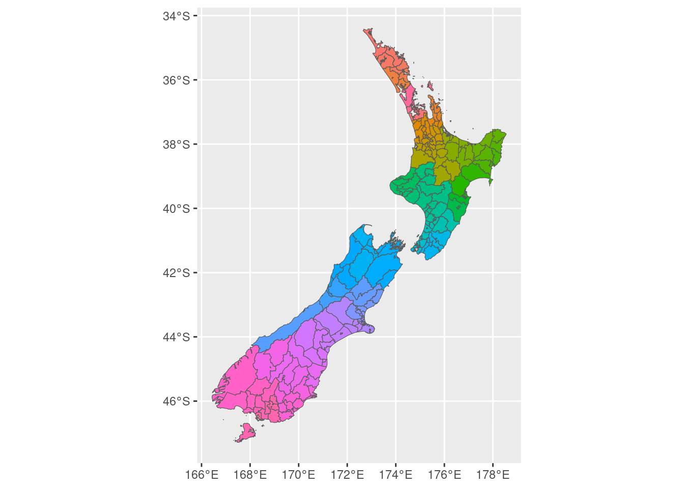
Here is a simple plot of the 257 wards coloured by their 2013 ward code to check that the modifications above worked as expected.
8.2 Exploring Simulated Incidence Data
Now let’s import some simulated incidence data and explore this. We will plot the observed cases and observed SIRs.
##   area_code            area_name observed  expected  covariate
## 1      3102 Onekawa-Tamatea Ward        4 10.354585 -0.4917083
## 2      5803         Cheviot Ward        4  4.262939 -0.1641180
## 3      3903        Feilding Ward        5  8.189436 -0.1674871
## 4      4403         Eastern Ward        5  5.941533 -0.5961955
## 5      1701        Pirongia Ward       10  6.245884  0.1429696
## 6      3005      Kahuranaki Ward       13 18.697521 -0.3818318
# Combine with sf
map <- map %>%
mutate(WARD2013 = as.integer(WARD2013)) %>%
left_join(
sim.data %>%
select(-area_name),
by = c("WARD2013" = "area_code")
)
# Compute the observed (raw) SIR
map <- map %>%
mutate(SIR = observed / expected)
# Create a modified data set for plotting
dat <- map %>%
# Truncate raw SIR and observed values
mutate(
SIR = case_when(
SIR > 4 ~ 4,
SIR < 0.25 ~ 0.25,
TRUE ~ SIR
),
observed = ifelse(observed > 150, 150, observed)
)
# Fill colours for observed and SIR variables
Fill.colours.obs <- c(grey(seq(1, 0, -0.2)), grey(0))
Fill.colours.SIR <- c("#2C7BB6", "#2C7BB6", "#ABD9E9", "#FFFFBF", "#FDAE61", "#D7191C",
"#D7191C")
# Values corresponding to the fill colours
Fill.values.obs <- c(seq(0, 150, 30), max(map$observed)) # Solid black for obs > 150
Fill.values.SIR <- c(log2(0.25), seq(log2(1/1.5), log2(1.5), length = 5), log2(4))
# Note: we use logged values for the SIR so that the colour gradient is linear
# Define the map border
map.border <- map %>%
select() %>% # Ignore everything except the geometry
summarise() # Dissolves the ward boundaries into one large region
# Common components of each map
gg.base <- ggplot(dat, aes(geometry = geometry)) +
guides(fill = guide_colourbar(barwidth = 15, position = "bottom")) +
theme_void()
# Add unique layers
gg.obs <- gg.base +
geom_sf(data = map.border, colour = "black", fill = "grey30", linewidth = 0.8) +
geom_sf(colour = NA, aes(fill = observed)) +
scale_fill_gradientn("",
colours = Fill.colours.obs,
values = rescale(Fill.values.obs),
limits = range(Fill.values.obs)
) +
ggtitle("Observed cases")
gg.SIR.raw <- gg.base +
geom_sf(data = map.border, colour = "black", fill = "grey30", linewidth = 0.8) +
geom_sf(colour = NA, aes(fill = log2(SIR))) +
scale_fill_gradientn("",
colours = Fill.colours.SIR,
values = rescale(Fill.values.SIR),
limits = range(Fill.values.SIR),
breaks = seq(-2, 2),
labels = round(2^seq(-2, 2), 3)
) +
ggtitle("Observed SIR")
# Render the plots
grid.arrange(gg.obs, gg.SIR.raw, nrow = 1)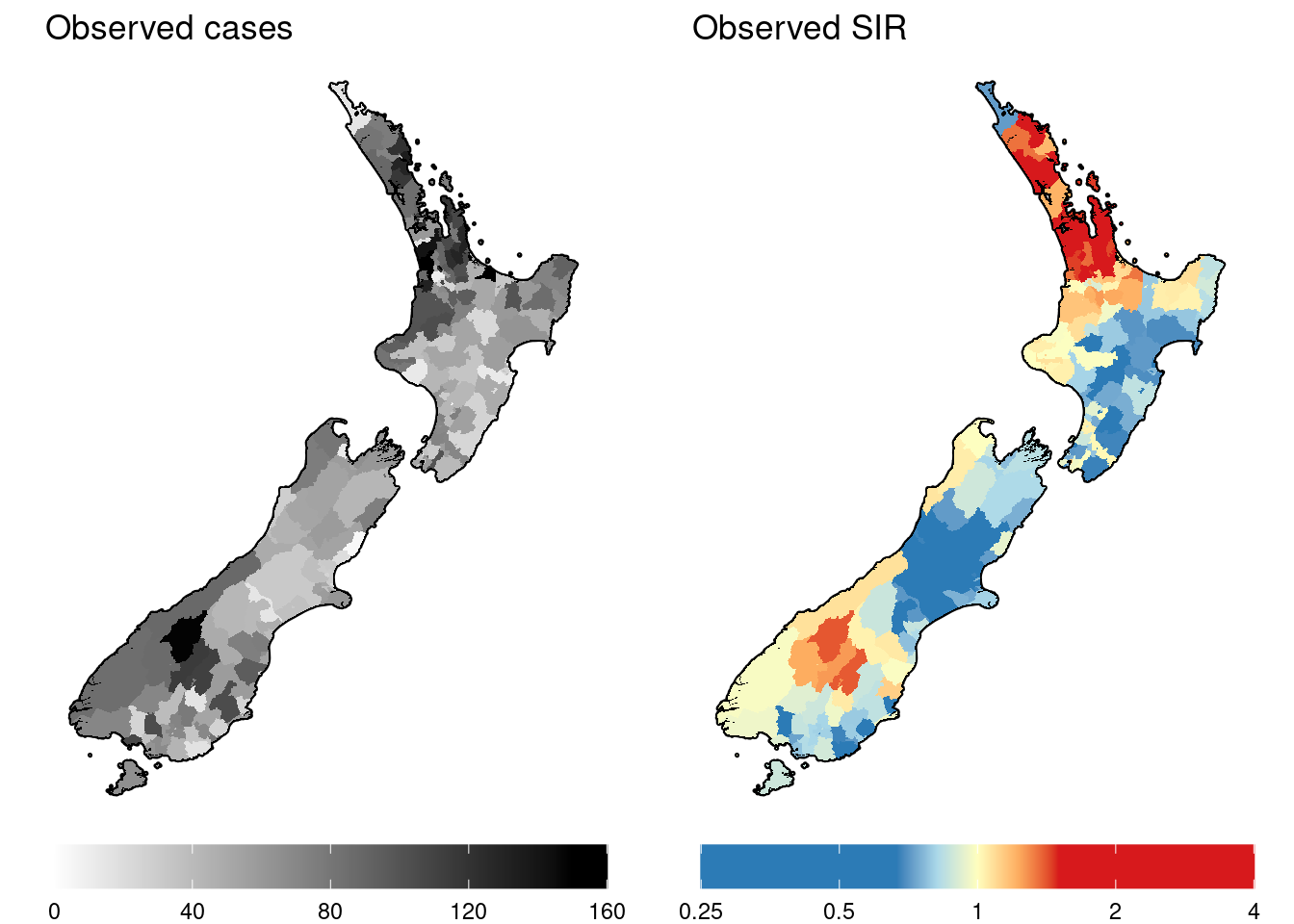
8.3 Fitting a Bayesian model to the Incidence Data
As with the simulated incidence data for Queensland, it is difficult to determine what spatial patterns exist from the raw data. Now it is time to fit a statistical model in order to estimate the (log) risk surface and the covariate and spatial random effects that compose it.
For this example, we will fit the BYM model (refer to Section 5.2.1). First, we compute the spatial adjacency data using the spdep package. The resulting object is a list which contains the same information as a spatial weights matrix (namely which areas are neighours of each area, and the corresponding weights), just in a different format. (For reasons explained below, there is no need to compute the corresponding spatial weights matrix.)
There are two areas with no immediately adjacent neighbours. The nearest neighbours will be used instead. These neighbours can be determined by computing the matrix of distances between each pair of areas as demonstrated earlier (see Sections 5.2.4 and 7.1). For the sake of brevity, these two nearest neighbours have been pre-determined; the IDs are hard-coded below. The following code updates this adjacency data list.
# Which areas have no neighbours?
no.neighbours <- which(adj.data$num == 0)

# Areas closest to these areas (based on nearest distance)
nearest.area <- c(243, 60)

# Recipricate areas with no neighbours and new neighbours for symmetry
nearest.area.r <- c(no.neighbours, nearest.area)
no.neighbours.r <- c(nearest.area, no.neighbours)

# Update adjacent neighbours
for(i in length(no.neighbours.r):1){
    # Cumulative sum of of neighbours
    if(no.neighbours.r[i] == 1){
        cumsum <- 0
    }else{
        cumsum <- sum(adj.data$num[1:no.neighbours.r[i]])
    }
    # Add neighbour after this index
    if(cumsum == 0){
        adj.data$adj <- c(nearest.area.r[i], adj.data$adj)
    }else if(cumsum == length(adj.data$adj)){
        adj.data$adj <- c(adj.data$adj, nearest.area.r[i])
    }else{
        adj.data$adj <- c(adj.data$adj[1:cumsum], nearest.area.r[i],
            adj.data$adj[(cumsum+1):length(adj.data$adj)])
    }
    # Update number of neighbours
    adj.data$num[no.neighbours.r[i]] <- adj.data$num[no.neighbours.r[i]] + 1
}

# Update weights
adj.data$weights <- c(adj.data$weights, rep(1, length(no.neighbours.r)))
Now we are ready to fit the model. Assuming some weakly informative priors, we will fit the following model:
\[Y_i \sim \mbox{Po}\left(E_i e^{\mu_i}\right)\] where \(Y_i\) and \(E_i\) are the observed and expected counts respectively, and \[ \mu_i = \beta_0 + \beta_1 x_i + S_i + U_i \\ \beta_0 \sim \mathcal{N}(0, 100) \\ \beta_1 \sim \mathcal{N}(0, 100) \\ S_i \mid \bm{S}_{\smallsetminus i} \sim \mathcal{N}\left(\frac{\sum_j{w_{ij}s_j}}{\sum_j{w_{ij}}}, \frac{\sigma_S^2}{\sum_j{w_{ij}}}\right) \\ U_i \sim \mathcal{N}\left(0, \sigma_U^2\right) \\ \sigma_S \sim HN(0, 10) \\ \sigma_U \sim HN(0, 10) \] where the Gaussian and half-Normal distributions are parameterised in terms of mean and variance.
This model can be fit using CARBayes (with the modification that the hyperprior for \(\sigma_S\) and \(\sigma_U\) are inverse-Gamma instead of half-Normal). However, CARBayes only returns the sum \(S_i + U_i\) rather than seperate parameters, which limits the inference that can be made about the spatial random effect. Instead, we will use the software OpenBUGS to fit the BYM model, which allows this additional flexibility, at the cost of some computational efficiency. Unlike CARBayes, OpenBUGS uses a list of adjacency data rather than the corresponding spatial weights matrix to define the intrinsic CAR prior distribution for \(S_i\). (For a more detailed explanation of the following code, refer to the OpenBUGS example provided in Appendix A.3.)
# Define the model (OpenBUGS code)
model <- function(){
    for(i in 1:N){
        y[i] ~ dpois(E.mu[i])
        E.mu[i] <- E[i] * exp(mu[i])

        mu[i] <- beta.0 + beta.1 * x[i] + S[i] + U[i]
        U[i] ~ dnorm(0, tau.U)
    }
    beta.0 ~ dnorm(0, 0.01)
    beta.1 ~ dnorm(0, 0.01)

    S[1:N] ~ car.normal(adj[], weights[], num[], tau.S)
    tau.S <- pow(sigma.S,-1)
    sigma.S ~ dnorm(0, 0.1)%_%T(0,)

    tau.U <- pow(sigma.U, -1)
    sigma.U ~ dnorm(0, 0.1)%_%T(0,)
}

# Save model to a temporary location
fp.model <- file.path(tempdir(), "OpenBUGS Model 8.3.txt")
write.model(model, fp.model)

# Fixed values (input data)
y <- dat$observed       # Observed values
E <- dat$expected       # Expected values
x <- dat$covariate      # Covariate

# Initial values for stochastic parameters
set.seed(4321)
inits <- function() {list(
    beta.0 = 0,
    beta.1 = 0.5,
    S = rnorm(N, 0, 0.5),
    U = rep(0, N),
    sigma.S = 0.1,
    sigma.U = 1
)}

# MCMC parameters
M.burnin <- 20000       # Number of burn-in iterations (discarded)
M <- 5000               # Number of iterations retained (after thinning)
# Fit the model using OpenBUGS
MCMC <- R2OpenBUGS::bugs(
data = c(list(N = N, y = y, E = E, x = x), adj.data),
inits = inits,
parameters.to.save = c("beta.0", "beta.1", "S", "U", "sigma.S", "sigma.U"),
model.file = fp.model,
n.chains = 1,
n.burnin = M.burnin,
n.iter = M.burnin + M, # Total iterations
n.thin = 5,
DIC = FALSE,
)
# Store the list of parameters for convenience (ignore the other stuff in MCMC)
pars <- MCMC$sims.listThe posterior estimates of each parameter are stored in the object pars. Because this is the BYM model, we need to modify the parameters \(S\) and \(U\) to resolve the likelihood identifiability problem (refer back to Section 5.2.1). We also recreate the log-relative risk parameter.
# User-defined function to compute proportion of excess variation
get.psi <- function(S, U){
    sd.S <- sd(apply(S, 2, median))
    sd.U <- sd(apply(U, 2, median))
    psi <- sd.S / (sd.S + sd.U)
    return(psi)
}

# Compute proportion of excess variation
psi <- get.psi(pars$S, pars$U)

# Modify random effects
pars$S <- pars$S - psi * pars$U
pars$U <- pars$U + psi * pars$U

# Recreate mu (log-relative risk)
pars$mu <- pars$beta.0 + outer(pars$beta.1, x) + pars$S + pars$U
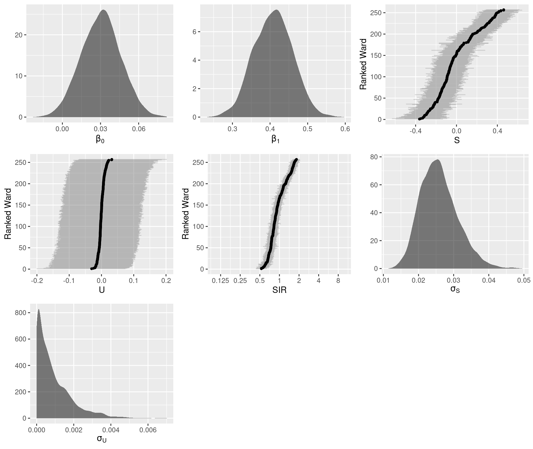
Graphical summaries of the marginal posterior distributions:
# Total number of sub-plots
gg.post <- vector("list", 7)

# Plot for beta_0
dat <- data.frame(val = pars$beta.0)
gg.post[[1]] <- ggplot(dat, aes(x = val)) +
    geom_density(fill = "black", alpha = 0.5, color = NA) +
    scale_x_continuous(expression(beta[0])) +
    scale_y_continuous("")

# Plot for beta_1
dat <- data.frame(val = pars$beta.1)
gg.post[[2]] <- ggplot(dat, aes(x = val)) +
    geom_density(fill = "black", alpha = 0.5, color = NA) +
    scale_x_continuous(expression(beta[1])) +
    scale_y_continuous("")

# Plot for S
dat <- pars$S
mean <- apply(dat, 2, mean)
CI.lower <- apply(dat, 2, quantile, probs = 0.025)
CI.upper <- apply(dat, 2, quantile, probs = 0.975)
rank <- order(order(mean))
dat <- data.frame(id = rank, mean, CI.lower, CI.upper)
gg.post[[3]] <- ggplot(dat, aes(x = id, y = mean)) +
    geom_pointrange(aes(ymin = CI.lower, ymax = CI.upper),
        alpha = 0.3, fatten = 0.1, colour = "grey50") +
    geom_point(size = 1) +
    scale_x_continuous("Ranked Ward", breaks = seq(0, N, 50)) +
    scale_y_continuous(expression(S)) +
    coord_flip()

# Plot for U
dat <- pars$U
mean <- apply(dat, 2, mean)
CI.lower <- apply(dat, 2, quantile, probs = 0.025)
CI.upper <- apply(dat, 2, quantile, probs = 0.975)
rank <- order(order(mean))
dat <- data.frame(id = rank, mean, CI.lower, CI.upper)
gg.post[[4]] <- ggplot(dat, aes(x = id, y = mean)) +
    geom_pointrange(aes(ymin = CI.lower, ymax = CI.upper),
        alpha = 0.3, fatten = 0.1, colour = "grey50") +
    geom_point(size = 1) +
    scale_x_continuous("Ranked Ward", breaks = seq(0, N, 50)) +
    scale_y_continuous(expression(U)) +
    coord_flip()

# Plot for relative risk (SIR)
SIR.labels <- c(0.125, 0.25, 0.5, 1, 2, 4, 8) # Ratio scale labels
dat <- pars$mu
mean <- apply(dat, 2, mean)
CI.lower <- apply(dat, 2, quantile, probs = 0.025)
CI.upper <- apply(dat, 2, quantile, probs = 0.975)
rank <- order(order(mean))
dat <- data.frame(id = rank, mean, CI.lower, CI.upper)
gg.post[[5]] <- ggplot(dat, aes(x = id, y = mean)) +
    geom_pointrange(aes(ymin = CI.lower, ymax = CI.upper),
        alpha = 0.3, fatten = 0.1, colour = "grey50") +
    geom_point(size = 1) +
    scale_x_continuous("Ranked Ward", breaks = seq(0, N, 50)) +
    scale_y_continuous("SIR", breaks = log(SIR.labels), labels = SIR.labels) +
    coord_flip(ylim = log(c(0.1, 10)))

# Plot for sigma.S
dat <- data.frame(val = pars$sigma.S)
gg.post[[6]] <- ggplot(dat, aes(x = val)) +
    geom_density(fill = "black", alpha = 0.5, color = NA) +
    scale_x_continuous(expression(sigma[S])) +
    scale_y_continuous("")

# Plot for sigma.U
dat <- data.frame(val = pars$sigma.U)
gg.post[[7]] <- ggplot(dat, aes(x = val)) +
    geom_density(fill = "black", alpha = 0.5, color = NA) +
    scale_x_continuous(expression(sigma[U])) +
    scale_y_continuous("")

# View combined plots
grid.arrange(gg.post[[1]], gg.post[[2]], gg.post[[3]], gg.post[[4]],
    gg.post[[5]], gg.post[[6]], gg.post[[7]], ncol = 3
)
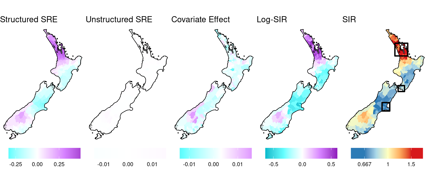
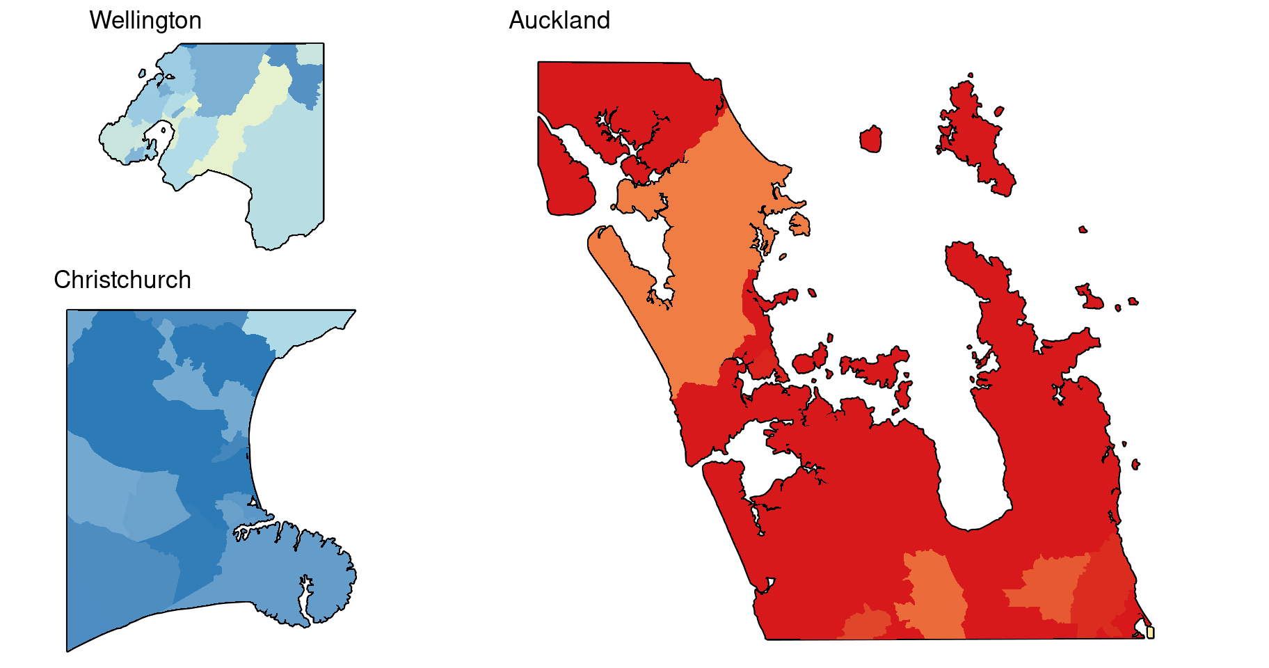
Now we decompose the log-risk surface (\(\mu_i\)) into its components: the structured and unstructured spatial random effects, \(S_i\) and \(U_i\) respectively, and the covariate effect, \(\beta_1 x_i\). For clarity, we combine the intercept with the structured spatial random effect.
First, we create the spatial data for map insets for 3 cities: Auckland, Wellington, and Christchurch. (This is the same process used in Section 7.1.)
# Create map inset borders
make.sf.rect <- function(x, y, CRS){
    rect <- c(x[1], y[1], x[2], y[1], x[2], y[2], x[1], y[2], x[1], y[1]) %>%
        matrix(ncol = 2, byrow = TRUE) %>%
        as.data.frame() %>%
        st_as_sf(coords = c("V1", "V2"), crs = CRS, agr = "constant") %>%
        summarise(geometry = st_combine(geometry)) %>%
        st_cast("POLYGON")
    return(rect)
}

map.Auckland.border <- make.sf.rect(x = c(174, 176), y = c(-37.5, -36), st_crs(map))
map.Wellington.border <- make.sf.rect(x = c(174.5, 175.5), y = c(-41.7, -41), st_crs(map))
map.Christchurch.border <- make.sf.rect(x = c(172, 173.2), y = c(-44, -43), st_crs(map))
Now we create the maps.
# Add posterior summaries of the model parameters to sf object
dat <- map %>%
    rename(raw.SIR = SIR) %>%
    mutate(
        S = apply(pars$S, 2, median) + median(pars$beta.0),
        U = apply(pars$U, 2, median),
        cov = median(pars$beta.1) * x,
        log.SIR = apply(pars$mu, 2, median),
        SIR = exp(log.SIR),
        # Truncate SIRs for plotting
        across(c(raw.SIR, SIR), ~ case_when(
            .x < 0.25 ~ 0.25,
            .x > 4  ~ 4,
            TRUE ~ .x
        ))
    )

# Fill colours
Fill.colours.linear <- c("#00bbcc", "#66ffff", "white", "#d580ff", "#8600b3")
Fill.colours.SIR <- c("#2C7BB6", "#2C7BB6", "#ABD9E9", "#FFFFBF", "#FDAE61", "#D7191C",
    "#D7191C")

# Range of linear components values (for consistent colour legend)
Lims <- dat %>%
    st_drop_geometry() %>%
    select(S, U, cov, log.SIR) %>%
    range() %>%
    abs()
Lims <- Lims[which.max(Lims)]
Fill.values.linear <- seq(-Lims, Lims, length = 5)

# Range of smoothed SIR values
Fill.values.SIR <- c(-2, seq(log2(1/1.5), log2(1.5), length = 5), 2)

Breaks.SIR <- c(0.5, 1/1.5, 1, 1.5, 2)

gg.base <- ggplot(data = NULL, aes(geometry = geometry)) +
    theme_void() +
    theme(legend.position = "bottom") +
    guides(fill = guide_colourbar(barwidth = 8))

gg.1 <- gg.base +
    geom_sf(data = map.border, fill = "grey30", color = "black", linewidth = 0.8) +
    geom_sf(data = dat, aes(fill = S), color = NA) +
    scale_fill_gradientn("",
        colours = Fill.colours.linear,
        values = rescale(Fill.values.linear, from = range(dat$S)),
        breaks = seq(-2, 2, 0.25)) +
    ggtitle("Structured SRE")

gg.2 <- gg.base +
    geom_sf(data = map.border, fill = "grey30", color = "black", linewidth = 0.8) +
    geom_sf(data = dat, aes(fill = U), color = NA) +
    scale_fill_gradientn("",
        colours = Fill.colours.linear,
        values = rescale(Fill.values.linear, from = range(dat$U)),
        breaks = seq(-2, 2, 0.01)) +
    ggtitle("Unstructured SRE")

gg.3 <- gg.base +
    geom_sf(data = map.border, fill = "grey30", color = "black", linewidth = 0.8) +
    geom_sf(data = dat, aes(fill = U), color = NA) +
    scale_fill_gradientn("",
        colours = Fill.colours.linear,
        values = rescale(Fill.values.linear, from = range(dat$cov)),
        breaks = seq(-2, 2, 0.01)) +
    ggtitle("Covariate Effect")

gg.4 <- gg.base +
    geom_sf(data = map.border, fill = "grey30", color = "black", linewidth = 0.8) +
    geom_sf(data = dat, aes(fill = log.SIR), color = NA) +
    scale_fill_gradientn("",
        colours = Fill.colours.linear,
        values = rescale(Fill.values.linear, from = range(dat$log.SIR)),
        breaks = seq(-2, 2, 0.5)) +
    ggtitle("Log-SIR")

gg.5 <- gg.base +
    geom_sf(data = map.border, fill = "grey30", color = "black", linewidth = 0.8) +
    geom_sf(data = dat, aes(fill = log2(SIR)), color = NA) +
    # Add map inset borders
    geom_sf(data = map.Auckland.border, colour = "black", fill = NA, linewidth = 1) +
    geom_sf(data = map.Wellington.border, colour = "black", fill = NA, linewidth = 1) +
    geom_sf(data = map.Christchurch.border, colour = "black", fill = NA, linewidth = 1) +
    scale_fill_gradientn("",
        colours = Fill.colours.SIR,
        values = rescale(Fill.values.SIR, from = range(log2(dat$SIR))),
        breaks = log2(Breaks.SIR),
        labels = round(Breaks.SIR, 3)) +
    ggtitle("SIR")

# View combined plots
grid.arrange(
    arrangeGrob(gg.1, gg.2, gg.3, gg.4, gg.5, nrow = 1)
)
Here are the map insets for the SIR estimates.
# Common components of each map
gg.base <- ggplot(dat, aes(geometry = geometry)) +
    scale_fill_gradientn("",
        colours = Fill.colours.SIR,
        values = rescale(Fill.values.SIR, from = range(log2(dat$SIR))),
        breaks = log2(Breaks.SIR),
        labels = round(Breaks.SIR, 3),
        limits = range(log2(dat$SIR))) +
    theme_void() +
    guides(fill = "none")

# Add visible layers for each map inset
gg.inset.Auckland <- gg.base +
    geom_sf(data = map.border %>% st_intersection(map.Auckland.border), colour = "black", fill = "grey30", linewidth = 0.8) +
    geom_sf(data = dat %>% st_intersection(map.Auckland.border), colour = NA, aes(fill = log2(SIR))) +
    ggtitle("Auckland")

gg.inset.Wellington <- gg.base +
    geom_sf(data = map.border %>% st_intersection(map.Wellington.border), colour = "black", fill = "grey30", linewidth = 0.8) +
    geom_sf(data = dat %>% st_intersection(map.Wellington.border), colour = NA, aes(fill = log2(SIR))) +
    ggtitle("Wellington")

gg.inset.Christchurch <- gg.base +
    geom_sf(data = map.border %>% st_intersection(map.Christchurch.border), colour = "black", fill = "grey30", linewidth = 0.8) +
    geom_sf(data = dat %>% st_intersection(map.Christchurch.border), colour = NA, aes(fill = log2(SIR))) +
    ggtitle("Christchurch")

# Render the plots
grid.arrange(
    arrangeGrob(gg.inset.Wellington, gg.inset.Christchurch, ncol = 1, heights = c(7, 11)),
    arrangeGrob(gg.inset.Auckland),
    ncol = 2, widths = c(1, 2)
)
Like the Queensland example in Section 7.3, we plot the observed and smoothed SIRs against the ranked SA2s to ascertain the effect of smoothing.
Breaks.SIR <- c(0.25, 0.5, 1/1.5, 1, 1.5, 2, 4)

# Add ranks
dat <- dat %>%
    mutate(rank = order(order(SIR)))

ggplot(dat) +
    geom_hline(yintercept = 1, linewidth = 1, colour = grey(0.3)) +
    geom_point(aes(x = rank, y = raw.SIR, shape = "Observed"), size = 2.5) +
    geom_point(aes(x = rank, y = SIR, shape = "Smoothed",
        colour = log2(SIR)), size = 2.5) +
    scale_x_continuous("Ranked SA2", expand = c(0.01, 0)) +
    scale_y_log10("", breaks = Breaks.SIR,
        labels = round(Breaks.SIR, 3),
        expand = c(0.01, 0.01)) +
    theme(panel.grid.minor.y = element_blank()) +
    scale_colour_gradientn("",
        colours = Fill.colours.SIR,
        values = rescale(Fill.values.SIR, na.rm = TRUE),
        breaks = log2(Breaks.SIR),
        labels = round(Breaks.SIR, 3),
        limits = range(Fill.values.SIR)
    ) +
    scale_shape_manual("",
        breaks = c("Observed", "Smoothed"),
        values = c("Observed" = 17, "Smoothed" = 16)
    ) +
    guides(colour = guide_colourbar(barheight = unit(8, "cm")))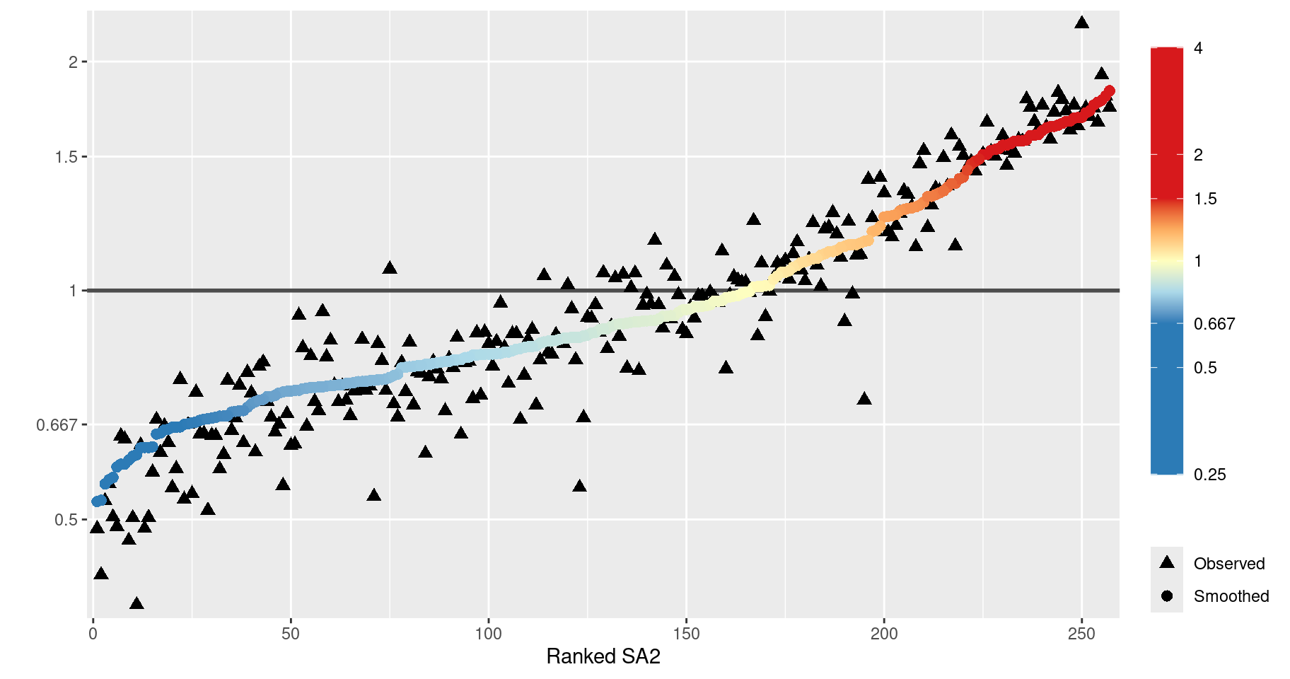
Note that there appears to be less smoothing occurring here than in the Queensland example in Section 7.3.