Chapter 4 Introduction to Spatial Models and CARBayes
4.1 Spatial Models and Data
A spatial model is:
- A model that allows for location, whether a geocoded coordinate or an area.
- Provides insight into geographic variations in disease risk.
We shall focus exclusively on models for areas.
Spatial models are useful for:
- Disease mapping: to estimate the true relative risk of a disease of interest across a geographical study area.
- Disease clustering: to assess whether a disease map is clustered and where the clusters are located; and estimate disease incidence around a putative hazard source (focused clustering).
- Ecological analysis: analysis of geographical distribution of disease in relation to explanatory covariates, usually at an aggregated spatial level.
Spatial data is typically autocorrelated and/or clustered. Spatial models attempt to account for this structure by including spatial autocorrelation. Including spatial autocorrelation is important because:
- otherwise the models assume spatial independence between areas (usually not realistic);
- this can cause bias in the results; and
- it can adjust for important influences.
To put this into perspective, ignoring spatial autocorrelation is akin to ignoring the order of time-series data.
There are many ways to create a spatial model to include spatial autocorrelation. This choice is influenced by the type and characteristics of the data. E.g.
- x-y coordinates versus area location
- assumed underlying disease processes
Examples of spatial models include:
- Kriging
- Empirical Bayes
- Fully Bayesian
This course focuses on fully Bayesian spatial models.
4.2 Fully Bayesian Spatial Models
The following Bayesian spatial model is a widely-used “natural model for disease mapping” (Best, Richardson, and Thomson 2005):
\[\begin{align*} \text{Stage 1}: \hspace{3em} & y_i \sim \text{Poisson}\left(E_i \theta_i \right) \\ \text{Stage 2}: \hspace{3em} & \log\left(\theta_i\right) = \text{intercept} + R_i \\ \text{Stage 3}: \hspace{3em} & \text{intercept} \sim p(\text{intercept}|\text{hyper-parameters}) \\ & R_i \sim p(R_i|\text{hyper-parameters}) \end{align*}\]
for \(i=1,\ldots,N\) areas.
The first stage is the likelihood model. The Poisson distribution is used because \(\left\{y_1, \ldots, y_N \right\}\) are count data for a typically rare or uncommon disease. \(E_i\) represents the expected cancer counts. \(\theta_i\) represents the standardised incidence ratio (SIR), also called the relative risk.
The second stage is an expression for the log-relative risk, (or log-SIR). This takes the form of a regression equation and typically includes an overall fixed effect (\(\text{intercept}\)), and a spatial random effect (\(R_i\)). This equation could also include covariates if available.
The third stage consists of the prior distributions for each of the unknown parameters, here \(\text{intercept}\) and \(R_i\). For parameters like the intercept, a weakly informative prior is usually appropriate (e.g. zero-mean Gaussian distribution with a large variance). For the spatial random effect (SRE) \(R_i\), the prior needs to take into account the spatial autocorrelation. Many priors have been devised to achieve this, and it is this prior which differentiates it from other spatial models. (Note: if the hyper-parameters in the third stage of the hierarchy are also treated as unknown, then a fourth stage can be added to specify hyperpriors for them.)
This is a generic three-stage hierarchical model - we will look at specific examples of this model in Chapter 5.
This model implies the following key assumptions:
- Individuals have independent propensity to disease (after allowing for observed/unobserved confounding variables). This allows events to be modelled via a likelihood approach. (Usually holds for non-infectious diseases; may hold for infectious if infectives are known.)
- Rather than assuming that the underlying at risk background intensity has a continuous spatial distribution, risk is assumed to be constant within each area. Any excess risk will be expressed beyond that described by expected counts. (Valid at appropriate scales of analysis. Not valid if area contains parts with 0 population.)
- The case-events are unique, i.e. occur as single spatially separate events. (Usually valid for relatively rare diseases.)
4.3 The Conditional Autoregressive (CAR) Distribution
One example of the prior that might be used for the spatial random effect is the [intrinsic] conditional autoregressive (CAR) distribution. This can be expressed through the following area-specific conditional distributions: \[ p(R_i | R_j, i \neq j, \sigma_R^2) \sim \mathcal{N}\left( \bar{\mu}_i, \sigma_i^2\right) \\ \bar{\mu}_i = \frac{1}{\sum_j w_{ij}}\sum_j R_j w_{ij} \\ \sigma_i^2 = \frac{\sigma_R^2}{\sum_j w_{ij}} \] where usually the weights are taken to be binary, first-order adjacency. This means: \[ w_{ij} = \begin{cases} 1 & \mbox{if areas } i \mbox{ and } j \mbox{ are adjacent}\\ 0 & \mbox{otherwise} \\ \end{cases}. \] The intrinsic CAR model can also be expressed through the joint density: \[p(\bm{R} | \sigma^2) \propto \exp\left\{ \frac{1}{2 \sigma^2} \sum_{i \neq j} w_{ij} \left( R_i - R_j\right)^2\right\}.\]
Note that this is an improper distribution, so it cannot be used for data (i.e. a likelihood), only random effects. The distribution also requires a constraint \(\sum_j R_j = 0\) so that the random effects are identifiable. (This is discussed in more detail in Section 5.2.1.)
The intrinsic CAR prior has the following advantages:
- Can be implemented in a wide choice of software
- Robust and often performs well
However, there are also some disadvantages:
- Designed for lattices, not irregular shapes and sizes
- The variance is influenced by the number of neighbours. When there are nested areas, they only have 1 neighbour
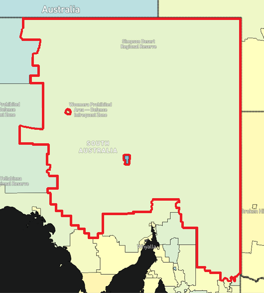
The following image demonstrates some of these potential drawbacks. The Outback has both nested SA2s, as well as the highest number of neighbours (21). This area is close to the size of Spain.
4.4 Defining Spatial Weights
The two obvious inputs into the spatial model are the observed cases, \(y_i\), and the expected cases, \(E_i\). Another input is the \(N \times N\) matrix of spatial weights, \(\bf{W}\), whose elements are \(w_{ij}\). When these weights are taken to be the binary, first-order adjacency weights, as described in the previous section, then the corresponding matrix is referred to as the adjacency [weights] matrix.
The spatial weights can be computed in R as demonstrated in Section 7.3. Another option is to use GeoDa. For a tutorial on using GeoDa, please see https://geodacenter.github.io/workbook/4a_contig_weights/lab4a.html. The key benefits of using GeoDa to construct an adjacency matrix are:
- Control (and ability to adjust neighbours)
- Connectivity insight (ability to see which areas constitute neighbours)
- Consistency (by using pre-assigned neighbours rather than determining them for each analyses)
4.5 Hyperpriors
Hyperpriors are priors on unknown parameters defining other priors higher up in the model hierarchy. For the CAR model above, it is common to have a hyperprior on the variance, \(\sigma_R^2\), since this parameter can have a large influence on the amount of spatial smoothing, and therefore fixing this parameter a priori can lead to poor or non-sensible results if not chosen very carefully.
Commonly used hyperpriors for this variance parameter are:
- \(\sigma_R^2 \sim \text{Inverse Gamma}(0, 0.01)\)
- \(\sigma_R^2 \sim \text{Uniform}(0, 20)\)
4.6 Computation: CARBayes
There are numerous software options for implementing a fully Bayesian spatial model like the intrinsic CAR model defined earlier. CARBayes (Lee 2013) is an R package that implements a range of well-known Bayesian spatial models. The advantages of CARBayes are:
- Easy
- Computationally fast to run
- Facilities a range of model types, including ones with discontinuities
The main disadvantages are the lack of flexibility and its “black box” nature of operation.
To implement the intrinsic CAR model in CARBayes, we use the function S.CARleroux(). This is because the intrinsic CAR model is a special case of the Leroux model when the parameter \(\rho\) is fixed at 1 (this is discussed in more detail in Section 5.2.3). The correct syntax looks something like this:
S.CARleroux(
    formula = y ~ offset(log(E)),
    data = data.frame(y = observed, E = expected),
    family = "poisson",
    W = W.mat,
    rho = 1,        # Fit intrinsic CAR model
    burnin = 10000,
    n.sample = 15000
)
Note W.mat is the spatial weights matrix. By default, the prior on the intercept is \(\mathcal{N}\left(0, 100000\right)\), while the hyperprior on the variance parameter is \(\mathcal{IG}\left(1, 0.01\right)\) which is an inverse-Gamma distribution parameterised in terms of shape and scale.
For documentation on using CARBayes, refer to:
- The CRAN documentation: https://cran.r-project.org/web/packages/CARBayes/CARBayes.pdf
- The CARBayes vignette: https://cran.r-project.org/web/packages/CARBayes/vignettes/CARBayes.pdf
4.7 CARBayes Demo 1
The following R code and data is adapted from the example on Andrew Lawson’s GitHub page: https://github.com/Andrew9Lawson/Bayesian-DM-code-examples/blob/master/SCcongen90_CARBayesRcode.txt
We first import the data provided by the maps library and convert it to a simple features (sf) object.
# Import data
SCcg90 <- read.csv("Downloaded Data/4.7 CARBayes Demo SCcg90.csv")

# Create a map of counties in South Carolina
SC.map <- maps::map(
    database = "county",
    regions = "South Carolina",
    plot = FALSE,
    fill = TRUE
) %>%
    # map2SpatialPolygons(IDs = SC.county$names)
    st_as_sf(SC.county, coords = c("lon", "lat"))  # Convert to sf
Next, we need to create the spatial weights matrix which forms part of the specification of the spatial random effect. The following R code shows how to compute the binary, first-order, adjacency weights matrix using the st_touches function.
# Create binary, first-order, adjacency spatial weights matrix
W <- st_touches(SC.map) %>%
    as.matrix() * 1
Note that if you are reading in a .gal file from GeoDa, then the following code could be used instead (note this uses the older spdep library):
W <- spdep::read.gal("map.gal", override.id = TRUE) %>%
    nb2mat(style = "B")  # Use neighbours list to create a spatial weights matrix
Now we fit a model using CARBayes. Here we fit the BYM model.
# MCMC parameters
M.burnin <- 10000       # Number of burn-in iterations (discarded)
M <- 1000               # Number of iterations retained

# Fit model using CARBayes
set.seed(444)          # For reproducability
MCMC <- S.CARbym(
    formula = obs ~ 1 + offset(log(exp)),
    data = SCcg90,
    family = "poisson",
    W = W,
    burnin = M.burnin,
    n.sample = M.burnin + M,    # Total iterations
    verbose = FALSE
)

# Broad summary of results
print(MCMC$summary.results)
## Mean 2.5% 97.5% n.sample % accept n.effective Geweke.diag
## (Intercept) 0.0339 -0.1162 0.1639 1000 32.2 248.2 0.4
## tau2 0.0205 0.0039 0.0629 1000 100.0 13.4 -2.7
## sigma2 0.0067 0.0014 0.0224 1000 100.0 29.0 -0.1## DIC p.d WAIC p.w LMPL loglikelihood
## 169.934473 3.210788 169.598476 2.657248 -84.866092 -81.756449In later examples, we will explore (and visualise) the output in more detail. Note that n.effective is the effective sample size (ESS), defined in Section 3.3.3. The terms relating to model fit were defined and described in Section 3.4.3.
4.8 CARBayes Demo 2
This example is adapted from the following article by Dr Paula Moraga: https://journal.r-project.org/archive/2018/RJ-2018-036/RJ-2018-036.pdf.
## [1] "geo" "data" "smoking" "spatial.polygon"## county cases population race gender age
## 1 adams 0 1492 o f Under.40
## 2 adams 0 365 o f 40.59
## 3 adams 1 68 o f 60.69
## 4 adams 0 73 o f 70+
## 5 adams 0 23351 w f Under.40
## 6 adams 5 12136 w f 40.59## county smoking
## 1 adams 0.234
## 2 allegheny 0.245
## 3 armstrong 0.250
## 4 beaver 0.276
## 5 bedford 0.228
## 6 berks 0.249We see that pennLC is a list object with the following elements:
geo: a table of county IDs, and the longitude and latitude of the centroid of each county;data: a table of number of lung cancer cases and population for each county, stratified by race, gender, and age group;smoking: a table of the proportion of smokers by county; andspatial.polygon: aSpatialPolygonsobject which can be used to create a map for Pennsylvania.
We now create a data frame with columns containing the county IDs, the observed and expected number of cases, the smoking proportions, and the SIRs.
# Add observed cases
pennLC$data <- pennLC$data %>%
    tibble() %>%
    group_by(county) %>%
    mutate(obs = sum(cases)) %>%
    ungroup()
We calculate the expected number of cases in each county using indirect standardisation. The expected counts in each county represent the total number of disease cases one would expect if the population in the county behaved the way the Pennsylvania population behaves.
# Add expected cases
pennLC$data <- pennLC$data %>%
    group_by(race, gender, age) %>%
    mutate(
        pop.strata = sum(population),
        cases.strata = sum(cases)
    ) %>%
    group_by(county) %>%
    mutate(
        expected = population * cases.strata / pop.strata,
        expected = sum(expected)
    ) %>%
    ungroup()

pennLC$data
## # A tibble: 1,072 × 10
## county cases population race gender age obs pop.strata cases.strata expected
## <fct> <int> <int> <fct> <fct> <fct> <int> <int> <int> <dbl>
## 1 adams 0 1492 o f Under.40 55 600471 3 69.6
## 2 adams 0 365 o f 40.59 55 212150 139 69.6
## 3 adams 1 68 o f 60.69 55 56371 134 69.6
## 4 adams 0 73 o f 70+ 55 65165 244 69.6
## 5 adams 0 23351 w f Under.40 55 2635605 25 69.6
## 6 adams 5 12136 w f 40.59 55 1481077 713 69.6
## 7 adams 5 3609 w f 60.69 55 476626 935 69.6
## 8 adams 18 5411 w f 70+ 55 823926 2394 69.6
## 9 adams 0 1697 o m Under.40 55 597435 3 69.6
## 10 adams 0 387 o m 40.59 55 185048 165 69.6
## # ℹ 1,062 more rowsWe can now disregard the variables except for the observed and expected counts for each county. Taking the ratio of the observed to expected counts, we obtain the observed SIR.
# Summarise observed and expected over county; add observed SIR
pennLC$data <- pennLC$data %>%
    select(county, obs, expected) %>%
    distinct() %>%
    mutate(SIR = obs/expected)

# Add the proportion of smokers variable
pennLC$data <- pennLC$data %>%
    left_join(pennLC$smoking, by = "county")
To create a chropleth map, we use the spatial information contained within pennLC$spatial.polygon. We’ll first modernise this object by converting it to a simple features (sf) object and then merge it with pennLC$data
# Create a sf object
map <- st_as_sf(pennLC$spatial.polygon, coords = c("lon", "lat")) %>%
    st_transform("+proj=longlat +datum=WGS84")   # Leaflet requires longlat/WGS84

# Add the data to the sf geometry
map <- cbind(map, pennLC$data)
Now we can visualise the any of the variables (observed, expected, SIRs, smokers proportions). We can create static maps, or dynamic interactive maps. Here we will create the latter using the leaflet package.
# Set colour palette
pal <- colorNumeric(palette = "YlOrRd", domain = map$SIR)

# Create interactive map
leaflet(map) %>%
    addTiles() %>%
    addPolygons(
        color = "grey",
        weight = 1,
        fillColor = ~pal(SIR),
        fillOpacity = 0.7
    ) %>%
    addLegend(
        pal = pal,
        values = ~SIR,
        opacity = 0.7,
        title = "SIR",
        position = "bottomright"
    )
We can improve the map by highlighting the counties when the mouse hovers over them, and showing information about the observed and expected counts, SIRs, and smoking proportions. We do this by adding the arguments highlightOptions, label and labelOptions to addPolygons(). Note that the labels are created using HTML syntax.
First, we create the text to be shown using the function sprintf() which returns a character vector containing a formatted combination of text and variable values and then applying htmltools::HTML() which marks the text as HTML. In labelOptions we specify the labels style, textsize, and direction. Possible values for direction are left, right and auto and this specifies the direction the label displays in relation to the marker. We choose auto so the optimal direction will be chosen depending on the position of the marker.
# Labels
labels <- sprintf(
    "<strong>%s</strong><br/>Observed: %s <br/>Expected: %s
    <br/>Smokers proportion: %s <br/>SIR: %s",
    map$county,
    map$obs,
    round(map$expected, 2),
    map$smoking,
    round(map$SIR, 2)
) %>%
    lapply(htmltools::HTML)

# Create interactive map
leaflet(map) %>%
    addTiles() %>%
    addPolygons(
        color = "grey",
        weight = 1,
        fillColor = ~pal(SIR),
        fillOpacity = 0.7,
        highlightOptions = highlightOptions(weight = 4),
        label = labels,
        labelOptions = labelOptions(
            style = list("font-weight" = "normal", padding = "3px 8px"),
            textsize = "15px",
            direction = "auto"
        )
    ) %>% addLegend(
        pal = pal,
        values = ~SIR,
        opacity = 0.7,
        title = "SIR",
        position = "bottomright"
    )
Now we can examine the map and see which areas have
- SIR = 1 which indicates observed cases are the same as expected,
- SIR > 1 which indicates observed cases are higher than expected,
- SIR < 1 which indicates observed cases are lower than expected.
This map gives a sense of the disease risk across Pennsylvania. However, observed (raw) SIRs may be misleading and insufficiently reliable in counties with small populations. In contrast, model-based approaches enable the incorporation of covariates and borrow information from neighbouring counties to improve local estimates, resulting in the smoothing of extreme values based on small sample sizes.
The paper which this example is based on uses INLA (Rue, Martino, and Chopin 2009) to fit the model. But we will use CARBayes instead.
# Create binary, first-order, adjacency spatial weights matrix
W <- st_touches(map) %>%
    as.matrix() * 1

# MCMC parameters
M.burnin <- 10000       # Number of burn-in iterations (discarded)
M <- 5000               # Number of iterations retained

# Fit BYM model using CARBayes
set.seed(111)          # For reproducability
MCMC <- S.CARbym(
    formula = obs ~ 1 + offset(log(expected)),
    data = map,
    family = "poisson",
    W = W,
    burnin = M.burnin,
    n.sample = M.burnin + M,    # Total iterations
    verbose = FALSE
)

# Broad summary of results
print(MCMC$summary.results)
## Mean 2.5% 97.5% n.sample % accept n.effective Geweke.diag
## (Intercept) -0.0530 -0.0830 -0.0229 5000 46.1 638.4 -2.5
## tau2 0.0127 0.0035 0.0320 5000 100.0 75.5 2.2
## sigma2 0.0049 0.0018 0.0111 5000 100.0 143.6 -1.7To obtain the modelled SIR, we need to divide the fitted values by the expected values.
Because we have a posteiror sample size of M = 5000 iterations, SIR is a \(M \times N\) matrix where \(N = 67\) is the number of counties. To visualise these estimates on the map, we will plot the median, and then add the 2.5th and 97.5 percentiles to the information that pops up when you hover the mouse over an area. We use RR to denote relative risk, which is the smoothed SIR (specifically, the median of the smoothed SIR), to distinguish it from the observed SIR. The posterior probability of the relative risk being greater than 1 (i.e. the proportion of MCMC iterations where the smoothed SIR is greater than 1) is also included, denoted by PP (this statistic is revisited in Section 11.1).
# Add summary statistics of the posterior SIR to map
map$SIR.50 <- apply(SIR, 2, median)
map$SIR.025 <- apply(SIR, 2, quantile, 0.025)
map$SIR.975 <- apply(SIR, 2, quantile, 0.975)
map$PP <- apply(SIR, 2, function(x) length(which(x > 1))) / M

# Optional: Update colour palette (harder to compare risk surfaces)
# pal <- colorNumeric(palette = "YlOrRd", domain = map$SIR.50)

# Update labels
labels <- sprintf(
    "<strong> %s </strong> <br/> Observed: %s <br/> Expected: %s <br/>
    Smoker proportion: %s <br/>SIR: %s <br/>RR: %s (%s, %s) <br/>PP: %s",
    map$county,
    map$obs,
    round(map$expected, 2),
    map$smoking,
    round(map$SIR, 2),
    round(map$SIR.50, 2),
    round(map$SIR.025, 2),
    round(map$SIR.975, 2),
    round(map$PP, 3)
) %>%
    lapply(htmltools::HTML)

# Create interactive map
leaflet(map) %>%
    addTiles() %>%
    addPolygons(
        color = "grey",
        weight = 1,
        fillColor = ~pal(SIR.50),
        fillOpacity = 0.7,
        highlightOptions = highlightOptions(weight = 4),
        label = labels,
        labelOptions = labelOptions(
            style = list("font-weight" = "normal", padding = "3px 8px"),
            textsize = "15px",
            direction = "auto"
        )
    ) %>%
    addLegend(
        pal = pal,
        values = ~SIR.50,
        opacity = 0.7,
        title = "Relative Risk",
        position = "bottomright"
    )